Assessing non-additive effects in GBLUP model

Abstract

Understanding non-additive effects in the expression of quantitative traits is very important in genotype selection, especially in species where the commercial products are clones or hybrids. The use of molecular markers has allowed the study of non-additive genetic effects on a genomic level, in addition to a better understanding of its importance in quantitative traits. Thus, the purpose of this study was to evaluate the behavior of the GBLUP model in different genetic models and relationship matrices and their influence on the estimates of genetic parameters. We used real data of the circumference at breast height in Eucalyptus spp and simulated data from a population of F2. Three commonly reported kinship structures in the literature were adopted. The simulation results showed that the inclusion of epistatic kinship improved prediction estimates of genomic breeding values. However, the non-additive effects were not accurately recovered. The Fisher information matrix for real dataset showed high collinearity in estimates of additive, dominant, and epistatic variance, causing no gain in the prediction of the unobserved data and convergence problems. Estimates presented differences of genetic parameters and correlations considering the different kinship structures. Our results show that the inclusion of non-additive effects can improve the predictive ability or even the prediction of additive effects. However, the high distortions observed in the variance estimates when the Hardy-Weinberg equilibrium assumption is violated due to the presence of selection or inbreeding can converge at zero gains in models that consider epistasis in genomic kinship.

Introduction

Genomic selection has now become a common practice in breeding programs. Choosing inappropriate models of direct regression in the genome can have a great interpretive impact on understanding the genetic architecture of populations in genomic analyses (Vitezica et al., 2013) as well as in decision making in breeding programs.

Considering the modeling of quantitative traits, great progress has been made in the last century. Sir Ronald Fisher proposed one of the first genetic models. This model assumes that quantitative traits are controlled by an infinite number of unconnected loci, with small additive effects of the same magnitude that follow a normal common distribution and depend on the allelic frequency of a reference population (Fisher, 1918).

Cockerham (1954) proposed an extension of the Fisher’s model, suggesting the breakdown of epistatic components in the interaction of different types of loci, such as additive-additive, additive-dominant, dominant-additive and dominant-dominant. Other genetic ad hoc models have been proposed. For example, Hayman and Mather (1955) established the genetic values as function of the genotypic values of individuals, regardless of the allelic frequency of the reference population. This model is popularly known as the metric F-infinite. The greatest drawback of this model is that the variance components and genetic effects are not decomposed in orthogonality, which can lead to inappropriate conclusions regarding the populations’ genetic architecture (Kao and Zeng, 2002; Zeng et al., 2005).

In principle, these models are often used in traditional analyses of the decomposition of variance components (Brim and Cockerham, 1961; Lee et al., 1968; Stuber and Moll, 1971). Non-addictive effects were also included in QTL mapping analysis (Cockerham and Zeng, 1996). However, few studies have thoroughly investigated the decomposition of variance components and genetic effects in direct regression models in the genome (Vitezica, et al., 2013).

Genetic effects can be decomposed into three classes of effects: i) additive, ii) dominance, and iii) epistasis. Additive effects are considered linear effects of each allele that are fully inheritable over generations. Dominance effects reflect the genotypic curvature in the function of the interaction of alleles of the same locus. Finally, epistatic effects are additional deviations due to a combination of two or more genes, i.e., a lack of additivity of the genotypic values of two different genes (Falconer and Mackay, 1996; Zeng et al., 2005).

Different concepts of epistasis are found in the literature. Functional epistasis describes the molecular action of proteins or other gene products that interact with each other in metabolic routes. Compositional epistasis refers to the classical idea of epistasis in which an allele of a given locus interferes with the expression of another locus and is then restricted to the individual. Statistical epistasis is defined as an average deviation of the resulting combination of alleles at different loci in a population of genotypes. This latter type of epistasis is most studied in quantitative genetics by the number of loci involved in the adaptability of an individual. For this reason, it is almost impossible to estimate the compositional epistasis for all loci (Phillips, 2008).

Understanding the importance of additive, dominant, and epistatic genetic effects in breeding populations is a key factor in choosing the parents in crosses, promising populations in recurrent selection schemes and selecting clones in perennial species where the fixation of epistatic and dominant effects may be applicable.

In this sense, the efficiency of genetic breeding programs of plants has greatly increased the potential for the exploitation of non-additive effects. In recent years, due to the development of large-scale genotyping techniques, such as genotyping-by-sequencing (GBS) (Elshire et al., 2011) and the reduction of the cost of genotyping, there has been great interest in the use of techniques aimed at exploring genomic information with a focus on minimizing costs in breeding programs (Heslot and Mark, 2014).

A large scientific effort is being directed towards increasing the effectiveness of these programs with the use of genomic analytical methods. Currently, the use of these techniques goes from understanding the genetic architecture of human intelligence to understanding the genetic mechanisms associated with plant resistance against pathogens (Davies et al., 2011; Edae et al., 2014).

The widespread adoption of models considering additive effects has been proposed in several studies due to the simplicity and importance of genetic interpretations (Massman et al., 2012; Albrecht et al., 2014; Technow et al., 2014). Models assuming dominance and epistatic effects have been proposed (Su et al., 2012; Vitezica et al., 2013; dos Santos et al., 2016) but are still rarely used in plant breeding, despite strong evidence that these models are important in understanding the genetic architecture of quantitative traits (Carlborg and Haley, 2004). As mentioned above, all these genetic models vary with the addition or removal of genetic effects or in the form of relatedness estimations between individuals of a current population, which have shown relationships relative to a reference population (Zeng et al., 2005; Van Raden, 2008; Powell et al., 2010; de Los Campos et al., 2013).

The GBLUP (best linear unbiased genomic predictor) is the most adopted direct regression model in genome statistical analysis due to its simplicity of interpretation and flexibility of modeling; it is also less computationally intensive and genetically intuitive (Gianola et al., 2014). Although recently proposed (Van Raden, 2008), the foundation of this model was previously explained (Henderson, 1984). The GBLUP is a model similar to the animal BLUP model, but instead of estimating the relationship between individuals by pedigree, the relationships are estimated by molecular markers. For many years, the BLUP model was widely used in animal breeding and less popularly in plant breeding (Smith et al., 2005; Piepho et al., 2008). The addition of non-additive effects in mixed models was first proposed by Henderson (1985), but not yet in the BLUP model. The biggest disadvantage of using this model is that epistasis is based on average relatedness, not considering information directly on the DNA level. Using the GBLUP model, it is possible to estimate not only the additive effects of molecular markers but also the dominance and epistatic effects at the genomic level.

Non-additive genetic effects are important in breeding programs, especially for species which are clonally propagated, such as Eucalyptus (Costa E Silva et al., 2004). Despite the large number of studies that have attempted to estimate these effects directly with regression models in the genome, few studies have compared, through simulation studies and real data, the accuracy of genetic effect estimates considering the full (with additive and non-additive effects) and the reduced models (with only additive effects).

Currently, one of the major statistical-genetic models under study is the improvement and increased prediction efficiency with the GBLUP model (Gianola et al., 2014). Thus, the three main objectives of this study were to i) examine a GBLUP model considering the first-order epistatic effects and the variance estimates based on Fisher information matrix; ii) determine which is the most convenient relationship matrix structure for the model evaluated; iii) obtain advanced results in an exploratory simulation study of the genetic control of parametric values; and iv) validate the findings with the genotypic data and real phenotypes of the Eucalyptus spp gender culture of the company Fibria S.A.

Materials and Methods

Study by simulation

In the simulation stage study, the data were obtained via the QGene 4.3.1 software (Joehanes and Nelson, 2008). Forty QTL (quantitative trait loci) were simulated and distributed randomly in the genome: 20 QTLs of additive effects (a) and dominance (d) with effects equal to 5, and 20 other QTLs with epistatic effects of the additive-additive type (aa), additive-dominant (ad), and dominant-dominant (dd) effect of 2.5. The simulated population consisted of 500 individuals from an F₂ population with 10 chromosomes and an allelic frequency of 0.5.

At the end of the simulation, 500 genotypes were generated with 6080 simulated marks each. The simulated population parameters are shown in Table 1.

Table 1:Population parameter values used in the simulation process.

Study with real phenotypic and molecular data

All phenotypic data and SNP markers were provided by Fibria S.A. The data were from a population of hybrids derived from crosses between E. grandis, E. urophylla, and E. globulus. The population was evaluated in an unbalanced test with repetitions ranging from two to fourteen. The adopted experimental design was incomplete blocks with composite portions of a plant (single tree plot). The population was structured with 611 genotypes originating from 68 progenies.

The subjects were phenotyped at 24 months of age for the circumference at breast height (cm) (CAP). Parallel to the phenotyping process, the DNA of all tested plants was extracted. Genotyping was performed using the GBS technique proposed by Elshire et al. (2011), resulting in 49,201 SNPs. In low frequency marker alleles, there are certain restrictions in the kinship calculation (Endelman and Jannink, 2012). Thus, alleles were deleted with a frequency lower than 0.05 and higher than 0.95 in the construction of the molecular marker matrix, as well as markers with losses greater than 5%. After eliminating, the number of SNPs was reduced to 39,781. Lost markers were computed by the A.mat function, mean method of the rrBLUP package (Endelman, 2011) in the R software.

Statistical methods

In this paper, three classes of models were used: i) additive - GBLUP-A; ii) additive/dominant - GBLUP-AD, and iii) epistatic - GBLUP-EP. These models were adopted in the two stages of analysis, both with simulated data and the actual phenotypic data. Next, the general GBLUP model and variations I, II, and III will be described.

The general GBLUP model can be defined by the following equation:

$y=X\beta +Zg+e$     (Equation 1)

where the vector of phenotypic observations (y) is decomposed in the vector of fixed effects of the observations (Xβ), random effects (Zg), and error (e). The vector of fixed effects (Xβ)_{n x 1} is obtained from the incidence matrix of fixed effects (X)_{n x k} multiplied by the vector of fixed effects (β)_{n x 1}. The matrix of random genetic effects (Zg) is the multiplication of the incidence matrix of random genetic effects (Z)_{n x p} by the vector of random genetic effects (g)_{p × 1}. The error vector (e)_{n x 1} contemplates the error related to each observation. The n, k, and p indices are the number of phenotypic observations, fixed effects, and random genetic values, respectively.

Distributions of random effects are considered g ~ N (0, $G{\sigma }_g^2$ ) and e ~ N (0, $I{\sigma }_e^2$ ). The observations are considered as y ~ N (μ, V), where the matrix $V$ is structured by:

$Var(y)=ZGZ´{\sigma }_g^2+I{\sigma }_e^2=V$     (Equation 2)

where G is a matrix of genetic variance-covariance (genomic relationship matrix), $I{\sigma }_e^2$ is the residual variance-covariance matrix and V is the phenotypic variance-covariance matrix and μ = Xβ.

Genomic kinship structures

For each model, three additive relationship matrix structures (A) were used. The first is the A matrix proposed by VanRaden et al. (2008) (V):

$A=\frac{W_A{W}_A\text{'}}{2{\displaystyle \sum pq}}$ (Equation 3)

where p is the frequency of the favorable allele and q is the frequency of the unfavorable allele; W_A is the deviation matrix of encoded markers by two (2 favorable alleles), 1 (a favorable allele), and 0 (no favorable allele) centralized in 2 p (average of the favorable allele at a given locus); 2Σpq is the sum of the locus variances.

The second matrix A was proposed by Yang et al. (2010) (Y) as expressed below:

$A_{ij}=\{\begin{array}{c}\frac{1}{N}{\Sigma }_i\frac{(x_{ij}-2p_i)(x_{ik}-2p_i)}{2p_i{q}_i},i\ne j\\ 1+\frac{1}{N}{\Sigma }_i\frac{x_{ij}{}^2-(1+2p_i)x_{ij}+2p_i{}^2}{2p_i{q}_i},i=j\end{array}$     (Equation 4)

where A_ij is Yang’s unified kinship matrix, in which i is the position in the line of kinship in the matrix, j is the position in the kinship column in the matrix, and x_ij is the i-th element of the matrix X, which indicates how many favorable alleles (0.1 or 2) the j-th individual has in that considered locus. The setting of this matrix by the empirical formula was also proposed by Yang et al. (2010), as stated by the authors; it sought to eliminate the bias associated with the use of a finite number of loci.

$A_{ij}^{adj}=\left(1-\frac{\frac{1}{N}}{\mathrm{var}(A_{ij})}\right)$     (Equation 5)

The third matrix used was proposed by Meuwissen et al. (2011) (M):

$G=\frac{XX\text{'}}{N}+I*{10}^{-4}$     (Equation 6)

where N is the number of SNPs and X is the standard genotypic matrix with the element x_ij calculated from the following expression:

$x_{ij}=\frac{g_{ij}-2p_j}{\sqrt{2p_j\left(1-p_j\right)}}$     (Equation 7)

where g_ij is the number of alleles in the genotype (0, 1, and 2) and p_j is the allele frequency of the j-th allele.

As stated by the authors, this matrix is equivalent to the matrix of Yang et al. (2010), but without separately calculating the diagonal and with the addition of a constant (I10^-4) on the diagonal of the matrix to make it a positive definite.

The dominance matrices followed the same corrections of the additive, that is, to the array of VanRaden et al. (2008) using the equation proposed by Vitezica et al. (2013):

$D=\frac{W_D{W}_D\text{'}}{4{\displaystyle \sum {(pq)}^2}}$     (Equation 8)

$where{w}_i=\{\begin{array}{c}-2q^2\\ 2pq\\ -2p^2\end{array}forthegenotypes\{\begin{array}{c}{A}^1{A}^1\\ A^1{A}^2\\ A^2{A}^2\end{array}$     (Equation 9)

The matrix D employed in Yang et al. (2010) model used the heterogeneous allelic frequency expression

$D_{ij}=\frac{1}{N}{\displaystyle \sum _i{w}_i\text{'}{w}_i/4{(p_i{q}_i)}^2}$     (Equation 10)

The third matrix D in the model provided by Meuwissen et al. (2011) (M) was constructed according to the equation:

$D=\frac{W_{d}W{\text{'}}_d}{N}$     (Equation 11)

where $W_i=\{\begin{array}{c}-2{(1-p)}^2\\ 2pq\\ -2p^2\end{array}$ for the genotypes $\{\begin{array}{c}{A}^1{A}^1\\ A^1{A}^2\\ A^2{A}^2\end{array}$ , respectively, with N as the total number of markers.

The matrices of epistatic kinship were obtained by Hadamard’s product (#) as follows: A#A, A#D, D#D, as shown by Henderson (1985) in the case of kinship matrices estimated by pedigree.

Thus, the complete model incorporating additive and epistatic effects is described by:

$y=X\beta +Zu+Z\delta +Zuu+Zu\delta +Z\delta \delta +e$     (Equation 12)

In the additive model, the only genetic estimated value corresponds to the additive genetic value (u). Therefore, g = u and

$V=A{\widehat{\sigma }}_u^2+I{\sigma }_e^2$     (Equation 13)

In the additive/dominant model, the dominance deviation ( $\widehat{\delta }$ ) was incorporated in the model. Thus,

$g=u+\delta andV=A{\widehat{\sigma }}_u^2+D{\widehat{\sigma }}_{\delta }^2+I{\sigma }_e^2$     (Equation 14)

The epistatic model was built by the addition of additive-additive epistatic (uu), additive-dominant (uδ), and dominant-dominant (δδ) variables. Consequently,

$g=u+\delta +uu+u\delta +\delta \delta$     (Equation 15)

and the total phenotypic variance is given by:

$V=A{\widehat{\sigma }}_u^2+D{\widehat{\sigma }}_{\delta }^2+A\#A{\widehat{\sigma }}_{uu}^2+A\#D{\widehat{\sigma }}_{u\delta }^2+D\#D{\widehat{\sigma }}_{\delta \delta }^2+I{\sigma }_e^2$     (Equation 16)

The maximization of the restricted maximum likelihood function (REML) of all variance components for all models described above was performed using the expectation-maximization (EM) (Dempster, 1977) and the Fisher score (Longford, 1987) algorithms. All the programs were built in the R platform (R Development Core Team, 2011).

Correlations estimated in the study by simulation

The efficiency of the three models was evaluated by three measures. The first was the Pearson correlation $r_{g\widehat{g}}$ between real genetic values (parametric) with genetic values estimated by different models. The other statistic was the heritability coefficient, estimated by:

$h_{\widehat{g}y}^2=\frac{{\sigma }_{\widehat{g}}^2}{{\sigma }_{\widehat{g}}^2+{\sigma }_e^2}$     (Equation 17)

where ${\sigma }_{\widehat{g}}^2$ is composed of the variances related to the main isolated effects ( ${\widehat{\sigma }}_u^2$ and ${\widehat{\sigma }}_{\delta }^2$ + ${\widehat{\sigma }}_u^2$ ) and with the inclusion of the effects ${\widehat{\sigma }}_{uu}^2$ , ${\widehat{\sigma }}_{u\delta }^2$ , and ${\widehat{\sigma }}_{\delta \delta }^2$ . The variance components estimated by the analysis were compared with the parametric values.

Study with real data: crossed validation and correlations

The cross-validation method used was k-fold. The set of 611 observations was randomly divided into six data groups, five groups consisting of 100 observations each and the last group consisting of 111 observations. The screening process sequentially eliminated each group in turn to be used as a validation population. The remaining subjects were used as a training population. The process was repeated until all the groups were used as the validation population. The efficiency was estimated in two steps, similar to the procedures used in the study by simulation. The first was the Pearson correlation between predicted values of the validation group, with the estimated genetic values in the analysis considering the six groups (611 observations). It is noteworthy that for these estimates, the genetic values considering the six groups were only those estimated by the epistatic model. The second way of verifying the production efficiency was to use the heritability estimate ( $h_{\widehat{g}}^2$ ), which was also used in the simulation study. Since the real data of the parameters are unknown, the expected information matrix was provided by the negative inverse of the Hessian to estimate the errors of the estimate and its covariance. Accordingly, we used the EM algorithm, and after convergence, an additional step of the Fisher score was applied. The Fisher information matrix was estimated to assess the precision of the variance components. Thus, the estimates of the standard deviations of the variance components were obtained by

$s_{({\sigma }^2)}=\sqrt{diag(I_o})$     (Equation 18)

Where I_o is the expected information matrix obtained by the inverse of the negative of the Hessian matrix given by:

 

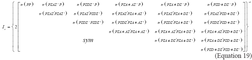
where $P=V^{-1}-V^{-1}X{(X\text{'}{V}^{-1}X)}^{-1}X\text{'}{V}^{-1}$ is the orthogonal projector.

Results

Simulation results

The variance components estimated by the GBLUP-A, GBLUP-AD, and GBLUP-EP models of the simulated dataset and the three kinship structures are shown in Table 2.

Table 2: Variance components of the simulated ( S ) and estimated data with the additive (GBLUP-A), additive-dominant (GBLUP-AD), and epistatic (GBLUP-EP) models, considering the kinship structures V, M, and Y.

The estimates of the variance components were similar for the three kinship matrices. However, in the epistatic model considering Yang’s matrix (Y), the component’s estimate ${\widehat{\sigma }}_{u\delta }^2$ was almost double in relation to the other kinship matrices approaching the parametric value. Despite this, the genetic variance estimated by this kinship structure in the epistatic model was similar to the others. There was no major change in the components of the additive and dominant variance when the epistatic effects were included in the model, which shows some orthogonality between these variance components.

In general, estimates of the variance components using the Y matrix showed a slightly greater magnitude relative to other matrices (Table 2). The kinship structures V and M showed very similar estimates to each other, which indicated that they captured the same information.

There was good accuracy in the additive genetic variance upon employing these kinship structures; however, the dominance variance almost doubled, and there was not good accuracy in the variance components related to epistasis (Table 2). For example, the epistatic component estimated with more efficiency ( ${\widehat{\sigma }}_{u\delta }^2$ = 10.53) was still very far from the simulated parametric value ( ${\widehat{\sigma }}_{u\delta }^2$ = 31.25). Considering the GBLUP-EP model, the Y matrix was the most efficient in the estimation of the variance components ${\widehat{\sigma }}_{u\delta }^2$ and ${\widehat{\sigma }}_{uu}^2$ ; however, these estimates were far from the parametric values. For the GBLUP-A and GBLUP-AD models, we noted the opposite effect: the V and M matrices produced results closer to the simulated values. It is possible that, except for the epistatic components, all components were overestimated for the magnitude of the parameters.

Considering the additive effects shown in Figure 1, there was no difference in the estimated causal regions for different models and matrix structures, i.e., the different matrix structures did not produce significant changes in the identification of additive genes. In addition, the inclusion of dominance and epistatic effects did not change the pattern of graphics, which agrees with the marginal change in the variance components.

Considering the dominance effects of the markers, it is also possible to confirm the same results previously reported, namely, that high coincidence was observed in the estimated dominance effect using different models and different dominance relationship matrices (Figure 2).

The accuracy of the predictions of the genetic values was verified by the correlation between simulated and predicted values (Table 3). It was observed that the different matrices of kinship had the same performance. Nevertheless, there was an increase in the accuracy of the estimates of the additive effects when the model incorporated the dominance and epistatic effects. Considering the dominance effects, there was virtually no change in the estimated accuracy when epistatic effects were included. However, when taking into account the total genetic effects, it was noted that the predictive accuracy increases when considering the inclusion of non-additive effects in the model ( $r_{g\widehat{g}}$ = 0.72-0.78). The accuracy in the estimation of epistatic effects was of lesser magnitude, which shows that the estimation of epistatic effects using matrices of epistatic kinship via direct products is not precise. It is noteworthy that the accuracy of the estimates of epistatic effects of the additive-dominant type was very similar for all matrices, although the estimate of the variance component was almost double for matrix Y. In general, matrices V and M estimated closer values in relation to the simulated value.

Table 3:Correlations of the simulated and estimated data considering the kinship structures V, M, and Y and estimated with additive (GBLUP-A), additive-dominante (GBLUP-AD), and epistatic (GBLUP-EP) models.

Table 4:Heritabilities of the simulated data (S) and estimated by the models with epistatic kinship structures V, M, and Y, using the additive (GBLUP-A), additive-dominant (GBLUP-AD) and epistatic (GBLUP-EP) models.

Table 4:Heritabilities of the simulated data (S) and estimated by the models with epistatic kinship structures V, M, and Y, using the additive (GBLUP-A), additive-dominant (GBLUP-AD) and epistatic (GBLUP-EP) models.

Heritabilities were overestimated in all possible configurations, especially the ones regarding the additive and dominant effects. For all the epistatic components except for the component $h_{u\delta }^2$ , all values obtained overestimated the heritability values. The GBLUP-EP model inflated the heritability estimates in the wide sense ( $h_{\widehat{g}}^2$ ) for all the kinship matrices, which ranged from 0.3254 for the V and M matrices to 0.3295 for matrix Y.

Real data results

The estimates of the variance components associated with the genetic analysis of the Eucalyptus spp population are shown in Table 5. It was noted that in the GBLUP-A model, there was little difference in the magnitude of the additive components of variance with the use of all tested kinship matrices. With the inclusion of the dominance effect (the GBLUP-AD model), a slight reduction in matrices M and Y and a greater reduction in matrix V in the magnitude of the estimates of the additive effects were observed on the expression of the CAP trait. In the same model, the standard deviation (SD) of the estimated ${\sigma }_{\delta }^2$ component was higher than actual value for the parameter, indicating the low precision of this estimate. With the addition of epistatic effects in the model, the value of estimates for the ${\widehat{\sigma }}_u^2$ component was reduced in relation to the other models tested, considering all kinship structures. However, this reduction was more evident in the Van Raden matrix.

Table 5:Variance components of the analysis of real data of the Eucalyptus spp estimated by the kinship structures V, M, and Y epistatic, with the additive (GBLUP-A), additive-Dominant (GBLUP-AD), and epistatic (GBLUP-EP) models.

Comparatively, the residual variance decreased pronouncedly when the non-additive effects were included in the model under the Van Raden matrix when compared to the other structures. In the case of the M and Y matrices, the inclusion of non-additive effects had little influence on the total variance, and the reduction in the residual variance was marginal. At first glance, one may assume that the Van Raden (V) structure would be the best choice. However, when observing the error associated with each of the estimates of non-additive genetic variances, there is great uncertainty and the inclusion of these effects becomes questionable. Furthermore, the drastic decrease in the estimation of the dominant and additive components upon the inclusion of epistatic effects reflects high covariance between these parameters in the model (Figure 3). In this graph, it is evident that there was high covariance between the estimates of variance components, and unlike what occurred with the simulated data, the inferences were highly compromised (Figure 4). In the latter case, the expected information matrices were practically diagonals, which resulted in less influence of the insertion of epistatic effects in the dominant and additive variances as well as gains in predictive accuracy. These observations agree with those found by Muñoz et al. in 2014.

Table 5 shows that the errors associated with non-additive components were much higher than the estimated values. However, considering that the Y and M matrices’ non-additive values were of low magnitude, the influence of these components in the overall analysis did not affect the results.

The low efficiency in estimating non-epistatic effects caused the Van Raden matrix to be slightly inferior in the prediction of phenotypic values in relation to Yang and Meuwissen’s matrix (Table 6). In general, the Meuwissen matrix was superior in predicting the phenotypic values and was the only one that positively included the non-epistatic effects. This result is reflected in the reduction of residues as the best predictive capacity considering all of the results of the 6-fold analysis.

Table 6: Correlation analysis of real data for the Eucalyptus spp estimated by the epistatic kinship structure models V, M, and Y, with the additive (GBLUP-A), additive-dominant (GBLUP-AD), and epistatic (GBLUP-EP) models.

The gains in accuracy considering the non-additive genetic effects may be misleading because they reflect only the results of a linear combination, which was not able to improve the predictability of the model in the phenotypic data. Moreover, in all cases, the predictions of epistatic effects per se were low and negative. This result shows that increasing the complexity of the model produced no gains in accuracy in the real data set as was observed as simulated data.

Discussion

The incorporation of non-additive effects may increase the prediction accuracy in the study of quantitative traits. The use of molecular markers with the GBLUP model allows for the direct use of these effects at the genomic level, mainly the dominance effects as shown by our results. Decomposition of variance components without the use of molecular markers requires structured populations with a known segregation pattern (pedigree), which allows for the isolation of genetic components of a non-addictive nature. These designs require significant spending on phenotyping and time, and they are not feasible in commercial breeding program schemes (Bernardo, 2010). Moreover, it is expected that the estimation of genetic parameters considering only pedigree information is biased and does not consider Mendelian segregation and the genetic link between individuals with unknown kinship. Thus, some studies in the literature report higher accuracy in estimating variance components when using a genomic relationship matrix (Muñoz et al., 2014; Bouvet et al., 2016).

Kinship matrix

As emphasized in the methodology, the phenotypic and genotypic data set was simulated considering the allelic frequency of 0.5 and the absence of inbreeding. In this condition, it was expected that the GBLUP models with the V and M structures would show similar results due to the mathematical expression of the kinship calculation, a fact that was confirmed by the results obtained in this study. However, there was variation in the estimates of the components between the V and M structures for the real data set, in which the allelic frequency was different from 0.5 and there was a strong deviation from the expected values by Hardy-Weinberg balance (only 7.15% markers presented Hardy-Weinberg equilibrium). Our results confirm those obtained by Meuwissen et al. (2011), who did not observe significant differences when using these M and Y kinship structures in a simulation procedure. However, these same authors state that they opted for the use of the M matrix, since it assigns a greater weight to low frequency alleles, which are causal alleles in the expression of quantitative traits. This statement, although intuitive from a genetic point of view, is limited from a mathematical one. As emphasized by Endelman (2011), in the formulation of the construction of the M and Y matrices, in situations with low frequency alleles, these matrices tend to have elements tending to infinity. Therefore, loci with an allelic frequency of less than 0.01 and greater than 0.91 are eliminated. These results suggest that significant differences are not expected when choosing matrices M or Y, especially with low inbreeding. Thus, the genetic information retrieved by these arrays is practically identical.

Yang et al. (2010) state that the Y matrix, proposed in their study, estimates the total genetic variance in a non-biased way, as the construction of this matrix occurs with a setting that eliminates the restriction of the use of a sample of finite size, a fact that is not valid for matrices V and M. Our results, however, did not confirm this statement, given that the estimates of the components of the Y matrix were the most distant of the simulated values in the GBLUP-EP model, even in ideal conditions of allelic frequency equal to 0.5 and Hardy-Weinberg equilibrium.

Decomposition of variance components

A desirable property for modeling is to obtain models that promote the decomposition of variance components and effects of orthogonal manner, that is, in the case of genetic models, where there are no confounding variables between the values of the components obtained by the decomposition of the total variance or the total genetic value. There are three situations in which this phenomenon may occur: i) the presence of linkage disequilibrium; ii) using incidence matrices without orthogonality; and iii) the presence of genotype by environment (Zeng et al., 2005; Gianola et al., 2014). In the GBLUP model, this restriction would be the lack of orthogonality related to the marker centered matrix (W), used for the construction of kinship matrices (Material and Methods). An even more serious problem is encountered in the construction of the epistatic kinship matrix, first suggested by Henderson (1985) and recently proposed by Su et al. (2012) in the GBLUP since this matrix is inconsistent with the metric proposed by Cockerham (1954).

In the first proposal by Henderson (1985), he only suggested the multiplication of the direct matrix; for example, the matrix AA is constructed by the direct product A#A instead of including the partial Kronecker product $(\otimes )$ or with the preparation of all pairwise combinations between the markers to thereby construct the epistatic orthogonal matrix (Kao and Zeng, 2002; Zeng et al., 2005). A limitation of this procedure is the high level of computational resources needed to obtain these matrices in hyper-parameterization conditions.

When epistatic models are adjusted, it is necessary to determine whether the assumptions of orthogonality are met. In the GWS context, the incidence matrix of the markers is assumed to belong to a binomial distribution with an average $2p$ and a variance $2p(1-p)$ . These two parameters are used for the construction of the kinship matrices V, M, and Y. In these situations, the SNPs (2, 1, 0) should segregate with probability $(p^2\mathrm{,2}p(1-p),q^2)$ . However, if there is selection and inbreeding in the population, the expected segregation is given by $[p^2(1+f)\mathrm{,2}p(1-p)(1-f),q^2(1+f)]$ _, where $f$ is the inbreeding coefficient or covariance between alleles. In such a scenario, there is no guarantee of orthogonality between the additive effects and dominance effects; consequently, the effects of epistasis are highly correlated. The orthogonality between dominance and additive effects comes from the assumption of the non-linear effect of a polynomial or just because of the residue from the lack of adjustment of a linear additive model (Cockerham, 1954).

For example, consider data from an SNP where there are 5 individuals with genotypes (2, 2, 1, 0, 0). It is easy to see that this SNP exhibits inbreeding and the allelic frequency is 0.5. Considering the dominance matrix, the expected result is W_d = (-0.5, -0.5, 0.5, -0.5, -0.5)^T and the additive vector is given by W = (1, 1, 0, -1, -1)^T. Therefore, the covariance between W and W_d is null and the orthogonal effects are guaranteed. However, changing from a 0 to 1 for this SNP changes the allelic frequency to 0.6 and the covariance between additive and dominance effects rises to 0.04. In order to ensure orthogonality in this frequency (0.6), SNPs coded as 2, 1, and 0 should follow a binomial distribution (or Hardy-Weinberg equilibrium) with probabilities of $[p^2=\mathrm{0.36,}2p(1-p)=\mathrm{0.48,}{q}^2=0.16]$ , respectively.

Thus, it is apparent that inbreeding population at an allelic frequency equal to 0.5 guarantees the orthogonality between different effects but frequencies different from 0.5 requires Hardy-Weinberg equilibrium. The lack of orthogonality may cause bias in the estimates of components of variance and problems with convergence. Our results demonstrate that in simulation conditions where the allele frequency is 0.5, all components were estimated orthogonally. This is clear because the behavior of the variance components did not change much when the model was minimal (purely additive) or maximum (main and epistatic effects). Moreover, the Hessian matrix showed a quasi-diagonal structure, resulting in faster convergence of the EM algorithm and low estimated variances. However, in the population of eucalyptus, which showed allelic frequencies ranging from 0.02 to 0.73 and in only 7.15% of the loci in Hardy-Weinberg equilibrium, the loss of orthogonality was evident when analyzing the changes in the variance components and structure of the Hessian matrix. With regard to this structure, the presence of high values in the off diagonal drastically alters the estimated error and may force the algorithm to exhibit Heywood cases and non-convergence.

Due to these problems in orthogonality, there was no predictive advantage for the real data when non-additive effects were used, and the marginal gain/loss regarding each effect only reflects a re-arrangement of linear combinations (Table 6). However, it is clear that if the population does not show inbreeding and a frequency of 0.5, the advantages of including non-additive effects in the model are evident, even if the latter effects and their variances are not well estimated due to imposed assumptions of the dominance of kinship and epistatic matrices (Hadamard product).

Problems with the lack of orthogonality in the decomposition of variance components have also been reported by Su et al. (2012) and Bouvet et al. (2016) using the GBLUP-EP model.

Analysis of Eucalyptus spp

This article is the first to use the GBLUP-EP model in the study of additive and non-additive components to the CAP trait in species of Eucalyptus spp. In addition, it evaluated the effectiveness of three kinship matrices that represented the constructs that appear frequently in the literature. The results revealed a predominance of additive effects in relation to other effects for any kinship matrix used. It was also observed a low contribution of the epistasis effects, as evidenced by the small magnitude of variance components and the heritability of these components (Table S1). These results, although unreliable according to previous descriptions, agree with the results obtained by other authors (Costa E Silva et al., 2004; Araujo et al., 2012), which, despite having used the BLUP model with pedigree information, also observed the predominance of additive effects in relation to others. Using marker data, Bouvet et al. (2016) also found a strong predominance of additive effects or the height trait in the species of Eucalyptus grandis.

It is noted that additive genetic variance, considering all kinship matrices, was reduced as other effects were added to the model, which shows that in less complex models, additive variance is inflated by non-additive effects when orthogonality is not guaranteed. These observations were also reported by Muñoz et al. (2014) and Bouvet et al. (2016). From the breeder’s point of view, these results suggest the importance of considering the analysis of the expected Fisher information matrix for the non-additive effects in the model; otherwise, the genetic parameters used in decision making will be compromised.

Based on these results, we conclude that the inclusion of non-additive effects in the model can improve predictive accuracy, but in populations that have been strongly influenced by selection or inbreeding, additive and non-additive effects are not properly orthogonal and may show a low accuracy of the variance components that does not reflect a real increase in predictive accuracy. The different kinship matrices produced similar results with regard to estimates of additive variance, but were poor in the estimation of non-additive variances. The ability of the epistatic model in improving estimates is questionable if some presuppositions of the Cockerham’s polynomial model are violated.

References

- Albrecht T, Auinger HJ, Wimmer V, Ogutu JO, et al. (2014). Genome-based prediction of maize hybrid performance across genetic groups, testers, locations, and years. Theor. Appl. Genet. 127: 1375-1386. http://dx.doi.org/10.1007/ s00122-014-2305-z
- Araujo JA, Borralho NM and Dehon G (2012). The importance and type of non-additive genetic effects for growth in Eucalyptus globulus. Tree Genet. Genomes 8: 327-337.http://dx.doi.org/10.1007/s11295-011-0443-x
- Bernardo R (2010). Breeding for quantitative traits in plants. 2nd edn. Stemma Press, Woodbury.
- Bouvet JM, Makouanzi G, Cros D and Vigneron P (2016). Modeling additive and non-additive effects in a hybrid population using genome-wide genotyping: prediction accuracy implications. Heredity (Edinb) 116: 146-157. http:// dx.doi.org/10.1038/hdy.2015.78
- Brim CA and Cockerham CC (1961). Inheritance of Quantitative Characters in Soybeans. Crop Sci. 1: 187-190. http:// dx.doi.org/10.2135/cropsci1961.0011183X000100030009x
- Carlborg O and Haley CS (2004). Epistasis: too often neglected in complex trait studies? Nat. Rev. Genet. 5: 618-625. http://dx.doi.org/10.1038/nrg1407
- Cockerham CC (1954). An extension of the concept of partitioning hereditary variance for analysis of covariances among relatives when epistasis is present. Genetics 39: 859-882.
- Cockerham CC and Zeng Z-B (1996). Design III with marker loci. Genetics 143: 1437-1456.
- Costa E Silva J, Borralho NMG and Potts BM (2004). Additive and non-additive genetic parameters from clonally replicated and seedling progenies of Eucalyptus globulus. Theor. Appl. Genet. 108: 1113-1119. http://dx.doi. org/10.1007/s00122-003-1524-5
- Davies G, Tenesa A, Payton A, Yang J, et al. (2011). Genome-wide association studies establish that human intelligence is highly heritable and polygenic. Mol. Psychiatry 16: 996-1005. http://dx.doi.org/10.1038/mp.2011.85
- de Los Campos G, Hickey JM, Pong-Wong R, Daetwyler HD, et al. (2013). Whole-genome regression and prediction methods applied to plant and animal breeding. Genetics 193: 327-345. http://dx.doi.org/10.1534/genetics.112.143313
- Dempster AP (1977). Maximum likelihood from incomplete data via the EM algorithm. J. R. Stat. Soc. B 39: 1-38.
- dos Santos JPR, Vasconcellos RC, Pires LPM, Balestre M, et al. (2016). Inclusion of Dominance Effects in the Multivariate GBLUP Model. PLoS One 11: e0152045. http://dx.doi.org/10.1371/journal.pone.0152045
- Edae EA, Byrne PF, Haley SD, Lopes MS, et al. (2014). Genome-wide association mapping of yield and yield components of spring wheat under contrasting moisture regimes. Theor. Appl. Genet. 127: 791-807. http://dx.doi.org/10.1007/ s00122-013-2257-8
- Elshire RJ, Glaubitz JC, Sun Q, Poland JA, et al. (2011). A robust, simple genotyping-by-sequencing (GBS) approach for high diversity species. PLoS One 6: e19379. http://dx.doi.org/10.1371/journal.pone.0019379
- Endelman JB (2011). Ridge regression and other kernels for genomic selection with R package rrBLUP. Plant Genome 4: 250-255. http://dx.doi.org/10.3835/plantgenome2011.08.0024
- Endelman JB and Jannink JL (2012). Shrinkage estimation of the realized relationship matrix. G3 (Bethesda) 2: 1405-1413. http://dx.doi.org/10.1534/g3.112.004259
- Falconer DS and Mackay TFC (1996). Introduction to Quantitative Genetics 4th edn. Longmans Green, Harlow.
- Fisher RA (1918). The correlation between relatives on the supposition of Mendelian inheritance. Trans. R. Soc. Edinb. 52: 399-433. http://dx.doi.org/10.1017/S0080456800012163
- Gianola D, Morota G and Crossa J (2014). Genome-enabled Prediction of Complex Traits with Kernel Methods: What Have We Learned? In Proceedings, 10th World Congress of Genetics Applied to Livestock Production Vancouver, Canada.
- Hayman BI and Mather K (1955). The description of genetic interactions in continuous variation. Biometrics 11: 69-82. http://dx.doi.org/10.2307/3001481
- Henderson CR (1984). Applications of Linear Models in Animal Breeding Models. 3rd edn. University of Guelph, Guelph.
- Henderson CR (1985). Best Linear Unbiased Prediction of Nonadditive Genetic Merits in Noninbred Populations. J. Anim. Sci. 60: 111-117.http://dx.doi.org/10.2527/jas1985.601111x
- Heslot N and Mark JJ (2014). Perspectives for genomic selection applications and research in plants. Crop Sci. 55: 1-12. http://dx.doi.org/10.2135/cropsci2014.03.0249
- Joehanes R and Nelson JC (2008). QGene 4.0, an extensible Java QTL-analysis platform. Bioinformatics 24: 2788-2789. http://dx.doi.org/10.1093/bioinformatics/btn523
- Kao CH and Zeng Z-B (2002). Modeling epistasis of quantitative trait loci using Cockerham’s model. Genetics 160: 1243-1261.
- Lee JA, Cockerham CC and Smith FH (1968). The inheritance of gossypol level in gossypium I. additive, dominance, epistatic, and maternal effects associated with seed gossypol in two varieties of Gossypium hirsutum L. Genetics 59: 285-298.
- Longford NT (1987). A fast scoring algorithm for maximum likelihood estimation in unbalanced mixed models with nested random effects. Biometrika 74: 817-827. http://dx.doi.org/10.1093/biomet/74.4.817
- Massman JM, Jung HJG and Bernardo R (2012). Genomewide selection versus marker-assisted recurrent selection to improve grain yield and stover-quality traits for cellulosic ethanol in maize. Crop Sci. 53: 58-66. http://dx.doi. org/10.2135/cropsci2012.02.0112
- Meuwissen THE, Luan T and Woolliams JA (2011). The unified approach to the use of genomic and pedigree information in genomic evaluations revisited. J. Anim. Breed. Genet. 128: 429-439. http://dx.doi.org/10.1111/j.1439-0388.2011.00966.x
- Muñoz PR, Resende MF, Jr., Gezan SA, Resende MDV, et al. (2014). Unraveling additive from nonadditive effects using genomic relationship matrices. Genetics 198: 1759-1768. http://dx.doi.org/10.1534/genetics.114.171322
- Phillips PC (2008). Epistasis--the essential role of gene interactions in the structure and evolution of genetic systems. Nat. Rev. Genet. 9: 855-867.http://dx.doi.org/10.1038/nrg2452
- Piepho HP, Mohring J, Melchinger AE and Buchse A (2008). BLUP for phenotypic selection in plant breeding and variety testing. Euphytica 161: 209-228. http://dx.doi.org/10.1007/s10681-007-9449-8
- Powell JE, Visscher PM and Goddard ME (2010). Reconciling the analysis of IBD and IBS in complex trait studies. Nat. Rev. Genet. 11: 800-805.http://dx.doi.org/10.1038/nrg2865
- Smith AB, Cullis BR and Thompson R (2005). The analysis of crop cultivar breeding and evaluation trials: an overview of current mixed model approaches. J. Agric. Sci. 143: 449-462. http://dx.doi.org/10.1017/S0021859605005587
- Stuber CW and Moll RH (1971). Epistasis in maize (Zea mays L.). 2. Comparison of selected with unselected populations. Genetics 67: 137-149.
- Su G, Christensen OF, Ostersen T, Henryon M, et al. (2012). Estimating additive and non-additive genetic variances and predicting genetic merits using genome-wide dense single nucleotide polymorphism markers. PLoS One 7: e45293.
- R Development Core Team (2011). R: A Language and Environment for Statistical Computing. R Foundation for Statistical Computing, Vienna.
- Technow F, Schrag TA, Schipprack W, Bauer E, et al. (2014). Genome Properties and Prospects of Genomic Prediction of Hybrid Performance in a Breeding Program of Maize. 197: 1343-1355.
- VanRaden PM (2008). Efficient methods to compute genomic predictions. J. Dairy Sci. 91: 4414-4423. http://dx.doi. org/10.3168/jds.2007-0980
- Vitezica ZG, Varona L and Legarra A (2013). On the additive and dominant variance and covariance of individuals within the genomic selection scope. Genetics 195: 1223-1230. http://dx.doi.org/10.1534/genetics.113.155176
- Yang J, Benyamin B, McEvoy BP, Gordon S, et al. (2010). Common SNPs explain a large proportion of the heritability for human height. Nat. Genet. 42: 565-569. http://dx.doi.org/10.1038/ng.608
- Zeng Z-B, Wang T and Zou W (2005). Modeling quantitative trait Loci and interpretation of models. Genetics 169: 1711-1725. http://dx.doi.org/10.1534/genetics.104.035857
Keywords:
Download:
Full PDF- Share This