Evaluation of genotype x environment interactions in cotton using the method proposed by Eberhart and Russell and reaction norm models
Accepted: November 30, -0001
Published: August 17, 2017
Genet.Mol.Res. 16(3): gmr16039726
DOI: 10.4238/gmr16039726
Abstract
Cotton produces one of the most important textile fibers of the world and has great relevance in the world economy. It is an economically important crop in Brazil, which is the world’s fifth largest producer. However, studies evaluating the genotype x environment (G x E) interactions in cotton are scarce in this country. Therefore, the goal of this study was to evaluate the G x E interactions in two important traits in cotton (fiber yield and fiber length) using the method proposed by Eberhart and Russell (simple linear regression) and reaction norm models (random regression). Eight trials with sixteen upland cotton genotypes, conducted in a randomized block design, were used. It was possible to identify a genotype with wide adaptability and stability for both traits. Reaction norm models have excellent theoretical and practical properties and led to more informative and accurate results than the method proposed by Eberhart and Russell and should, therefore, be preferred. Curves of genotypic values as a function of the environmental gradient, which predict the behavior of the genotypes along the environmental gradient, were generated. These curves make possible the recommendation to untested environmental levels.
Introduction
Upland cotton (Gossypium hirsutum L.r. latifolium Hutch.) produces one of the most important textile fibers of the world since it offers varied products of utility with great relevance in the Brazilian and world economy (Carvalho et al., 2015). It is an economically important crop in Brazil, which is the world’s fifth largest seed cotton producer, with 4.0 million tons produced in the 2015/2016 crop season and production is concentrated in the Brazilian Midwest primarily (CONAB, 2016). However, cotton has gained prominence in other regions of Brazil, such as the Northeast; this makes it difficult for breeders to develop genotypes with wide adaptability and stability to these regions due to the occurrence of genotype x environment (G x E) interactions.
The presence of G x E interactions is characterized by the differentiated genotype response to the variations of the environmental conditions, which can cause an alteration in the performance ordering of the genotypes in the environmental gradient (Falconer and Mackay, 1996). The G x E interactions can be expressed in different ways and with different intensities and are of fundamental importance in genetic evaluations (Resende, 2015). According to Robertson (1959), variance component of the G x E interactions can be deployed into a simple part from the interactions, explained by the change in genetic variation (variance heterogeneity) of the genotypes in different environments, and into a complex part from the interactions arising from a lack of genetic correlation between the genotype performance from one environment to another. This is the problematical part of the interactions, meaning that the good genotype in one environment may not be in another.
According to Resende (2007), a genotype is considered stable when it presents small variations in its overall behavior under various environmental conditions. Another important concept is the adaptability or responsiveness to environmental improvement. This concept is associated with the plasticity of genotypes. In these terms, an ideal genotype is one that responds predictably or proportionally to environmental stimulus.
There are several procedures to evaluate the effects of G x E interactions in plant breeding (van Eeuwijk et al., 2016). One of the main methods used in cotton is based on simple linear regression analysis, proposed by Eberhart and Russell (1966). This method considers the coefficients of linear regression of the phenotypic values from each genotype concerning the environmental index and the deviations of this regression to select genotypes with stability and adaptability to favorable and unfavorable environments.
Although widely used for recommending cotton genotypes, the method proposed by Eberhart and Russell presents a limitation to deal with unbalanced data, non-orthogonal experimental designs (incomplete blocks), and heterogeneity of variances between the various experimental sites, which are common situations in field experimentation. Moreover, such methodology assumes, in general, that the effects of genetic treatments are fixed, which is disadvantageous and inconsistent with the existing practice of the estimation of variance components and genetic parameters performed based on these experiments (Resende, 2007).
Current genetic assessment techniques involve the estimation of variance components and the prediction for genetic values simultaneously. The standard procedure for estimation of variance components is the restricted maximum likelihood method (REML), developed by Patterson and Thompson (1971) and the most widely used procedure for prediction of genetic values is the best linear unbiased prediction (BLUP) (Henderson, 1975). Therefore, the optimal genetic evaluation procedure refers to the use of these two methodologies together called REML/BLUP, also known as the mixed model methodology (Resende, 2007).
Under this approach, reaction norm models present excellent theoretical and practical properties (Kolmodin et al., 2002; Calus et al., 2004; Streit et al., 2012). The reaction norm model is a covariance function that allows assigning to each genotype random regression coefficients that predict the genotypic value as a function of the environmental gradient (Resende et al., 2014). Thus, each genotype will have a genotypic value for each environment, considering the G x E interactions. The reaction norm models can be adjusted via random regression models by REML/BLUP, making it possible to obtain curves of genotypic values associated with the different genotypes (Kirkpatrick et al., 1990).
Therefore, the goal of this study was to evaluate the G x E interactions in two important traits in cotton (fiber yield and fiber length) using the method proposed by Eberhart and Russell (simple linear regression) and reaction norm models (random regression).
Materials and Methods
Experimental data
Eight trials with upland cotton genotypes were conducted during the harvest 2008/2009 in the State of Mato Grosso, Brazil, in the following municipalities: Primavera do Leste, Pedra Preta, Campo Verde, Lucas do Rio Verde, Sapezal, Campo Novo dos Parecis, Nova Ubiratã, and Primavera do Leste II. The experimental design adopted consisted of randomized complete blocks with 16 treatments (BRS ARAÇA, BRS BURITI, BRS 286, FMT 701, FM 993, FM 910, DELTA OPAL, IPR JATAI, LD CV 05, LD CV 02, BRS CEDRO, NUOPAL, CNPA MT 05 1245, CNPA MT 04 2080, CNPA MT 04 2088, and BRS 293) with four replicated. Characteristics of each environment are shown in Table 1.
| Environment | Site | Altitude (m) | Latitude | Longitude | Annual rainfall (mm) | |
|---|---|---|---|---|---|---|
| 1 | Primavera do Leste | 636 | 15°33' | 54°17' | 1713 | |
| 2 | Pedra Preta | 850 | 16°37' | 54°28' | 1558 | |
| 3 | Campo Verde | 736 | 15°32' | 55°10' | 1529 | |
| 4 | Lucas do Rio Verde | 399 | 13°03' | 55°55' | 1970 | |
| 5 | Sapezal | 387 | 12°59' | 58°45' | 2082 | |
| 6 | Campo Novo dos Parecis | 564 | 13°40' | 57°53' | 1939 | |
| 7 | Nova Ubiratã | 396 | 13°00' | 55°15' | 1990 | |
| 8 | Primavera do Leste II | 636 | 15°33' | 54°17' | 1713 |
Table 1. Characteristics of the 8 environments evaluated in the Mato Grosso State, Brazil.
Cultural practices were the ones commonly used for growing cotton, including the use of herbicides for weed and pest control, according to the integrated management of pests recommended for the crop in the region. The experimental unit consisted of four 5.0 m long rows, spaced at 0.90 m at a density of 9 plants/m. The traits evaluated were: cotton fiber yield (FY, kg/ha) and fiber length (FL, mm) using the high volume instrument from the Laboratory of Fibers of the Embrapa Algodão.
Linear regression model proposed by Eberhart and Russell
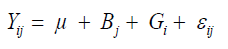
Firstly, it was applied the Kolmogorov-Smirnov test to verify if a probability distribution associated with the data set can be approximated by the normal distribution for each trait in each environment. After meeting this assumption, variance analysis for each trait in each environment was performed, based on the model in Equation 1:
 (Equation 1)
where Yij is the phenotypic value of the ith genotype evaluated in the jth block; Bj is the jth block effect assigned as fixed effect; Gi is the ith genotype effect assigned as a random effect; εij is the random error, to evaluate the experimental precision and homogeneity of residual variances.
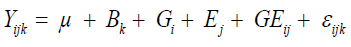
After verifying the homogeneity of residual variances, analysis of variance was performed considering all environments, based on the model in Equation 2:
 (Equation 2)
where Yijk is the phenotypic value of the ith genotype evaluated in the jth environment in the kth block; Bk is the kth block effect assigned as fixed effect; Gi is the ith genotype effect assigned as a random effect; Ej is the jth environment effect assigned as a fixed effect; GE(ij) is the G x E interaction effect assigned as a random effect; εijk is the random error, to evaluate the significance of the G x E interaction effect.
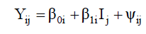
Adaptability and stability method proposed by Eberhart and Russell is based on the simple linear regression analysis that measures the performance of each genotype over environment variations according to Equation 3:
 (Equation 3)
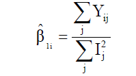
where Yij is the phenotypic value of the ith genotype in the jth environment; β0i is the linear coefficient of the ith genotype; βli is the regression coefficient that measures the ith genotype performance in the jth environment; Ij is the environment index that is estimated by Equation 4:
 (Equation 4)
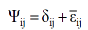
Besides, ψij is the random error, and it is decomposed by Equation 5:
 (Equation 5)
where δij is the regression deviation, and  is the mean experimental error. The estimative of mean square for adaptability and stability parameters based on Eberhart and Russell is estimated according to Equations 6 and 7, respectively:
 (Equation 6)
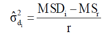 (Equation 7)
where MSDi is the mean square deviation of the ith genotype; is the residual mean square; r is the number of replication. The hypothesis are HO: β1i = 1 vs H1: β1i ≠ 1, and HO: σ2di = 0 vs H1: σ2di > 0. These hypotheses are evaluated by the Student t-test and the Fisher-Snedecor F-test, respectively.
The normality test and analyses of variance were performed in the Rbio software (Bhering, 2017) and the adaptability and stability model proposed by Eberhart and Russell was adjusted using the R Core Team (2016).
Reaction norm models adjusted by random regression
The reaction norm models adjusted by random regression (linear, quadratic, and cubic) are described below:
The linear model according to Equation 8 is:
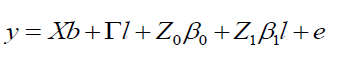 (Equation 8)
where y, b, l, and e are data vectors of fixed effects, block means over sites, fixed effects of environments or sites and random errors, respectively; β0 and β1 are coefficients of the intercept and linear of the random regression on the covariables, respectively; X and Γ are incidence matrixes for b and l, respectively; Z0: incidence matrix for β0 (containing 0 and 1’s); and Z1: matrix associating β0 to y (containing 0 and 1’s).
The quadratic model according to Equation 9 is:
 (Equation 9)
where y, b, l, and e are fixed effects, block means over sites, fixed effects of environments or sites and random errors, respectively; β0, β1, and β2 are coefficients of the intercept, linear, and quadratic of the random regression on the covariables, respectively; X and Γ are incidence matrixes for and , respectively; Z0: incidence matrix for β0 (containing 0 and 1’s); and Z1: matrix associating β0 and β2 to y (containing 0 and 1’s).
The cubic model according to Equation 10 is:
 (Equation 10)
where y, b, l, and e are fixed effects, block means over sites, fixed effects of environments or sites and random errors, respectively; β0, β1, and β2, and β3 are coefficients of the intercept, linear, quadratic, and cubic of the random regression on the covariables, respectively; X and Γ are incidence matrixes for b and l, respectively; Z0: incidence matrix for β0 (containing 0 and 1’s); and Z1: matrix associating β1, β2, and β3 to (containing 0 and 1’s).
The heritability according to the environmental gradient is estimated by Equation 11:
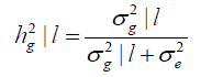 (Equation 11)
Genotype value of i at the j environmental level is defined by Equation 12:
 (Equation 12).
where d is the degree of equation and lj is the value of the covariate level.
Reaction norm models were adjusted using the phenotypic values centered on the general mean and environmental levels centered on the overall mean as a known covariate in a random regression model. These models were adjusted using the R Core Team (2016) software, lme4 package, lmer function (Bates et al., 2015). The significance of the coefficients of the reaction norm models was tested using the Wilks likelihood ratio test (LRT). The norms of reaction of the 16 genotypes in the common environment (l = 0) for each trait, along with the environmental gradient, were obtained using the R Core Team (2016) software, ggplot2 package (Wickham, 2009).
Results and Discussion
Regression model proposed by Eberhart and Russell
The HO hypothesis (the data follow a normal distribution) of the Kolmogorov-Smirnov test was rejected for the trait FY (P value < 0.05). The Box-Cox transformation (Box and Cox, 1964) was used for this trait. After meeting this assumption, variance analysis for each trait in each environment was performed to assess experimental precision and homogeneity of residual variances. According to Pimentel-Gomes (1985), the FY trait showed coefficients of variation ranging from low (below 10%) to moderate levels (between 10 and 20%), except for the environment 4, which had high coefficient of variation (between 20 and 30%), the FL trait had lower coefficients of variation. These values indicate, in general, high accuracy of the experimental results.
According to Hartley (1950), the maximum F-test is expressed by the ratio higher (MS residue)/lower (MS residue), equal to 4.59 for the FY trait and 3.31 for the FL trait and the hypothesis that there is homogeneity among the residual variances is not rejected at 1% probability. Thus, we proceeded to the joint analysis of variance shown in Table 2.
| Sources of variation | Degrees of freedom | Mean square | F calculated | |
|---|---|---|---|---|
| Blocks/Environments | 24 | 0.25 | | 0.66 | |
| Genotypes | 15 | 0.70 | | 6.81 | 5.57** | 8.72** |
| Environments | 7 | 15.12 | | 14.27 | |
| Genotypes x Environments | 105 | 0.13 | | 0.78 | 1.91** | 1.41* |
| Residue | 360 | 0.07 | | 0.55 | |
** and *significant at 1 and 5% probability by the Fisher-Snedecor F-test. Null hypothesis tested was that s2g = 0 and s2ge = 0, i.e., there is no genetic variability and G x E interactions.
Table 2. Summary of the joint analysis of variance for the traits fiber yield and fiber length (FY | FL) evaluated in 16 cotton genotypes cultivated in 8 environments in the Mato Grosso State, Brazil.
The genetic variance detected in the joint analysis of variance is equivalent to the genetic variance means in the various environments, subtracting the interactions. Joint analysis of variance showed significant effects for genotypes at 1% probability level for both traits, and for G x E interactions for FY, at 1% probability, and FL, at 5% probability. These results can be attributed to the edaphoclimatic differences between the sites (Table 1) and indicate the need for applying stability and adaptability methods to recommend the best genotypes. Similar results were obtained by Ng et al. (2013), Joy et al. (2012), and Campbell and Jones (2005), who also observed significant G x E interactions for the FY and FL traits..
The parameters of stability and adaptability estimated by the method of Eberhart and Russell are presented in Table 3. According to this method, the ideal genotype is one that has wide adaptability and high predictability (not significant and ); besides high phenotypic mean for the trait of interest. In this sense, the genotype FM 910 is the most suitable for the environment network (sites) used in this study, since they have a high phenotypic mean for FY and FL, as well as the ability to take advantage of the environmental stimulus, and have good predictability.
| Genotypes |  |
 |
 |
 |
|---|---|---|---|---|
| BRS ARAÇA | 1.96 | 31.10 | 0.95NS | 0.61NS | 0.01NS | 0.14NS | 90.37 | 26.18 |
| BRS BURITI | 2.12 | 31.49 | 0.72** | 1.65* | 0.02NS | 0.57++ | 80.43 | 50.24 |
| BRS 286 | 1.87 | 30.58 | 1.09NS | 0.71NS | 0.00NS | 0.03NS | 94.81 | 42.75 |
| FMT 701 | 2.09 | 30.27 | 1.01NS | 1.03NS | 0.00NS | -0.11NS | 93.53 | 89.69 |
| FM 993 | 2.14 | 31.19 | 1.30** | 0.71NS | -0.01NS | 0.01NS | 97.63 | 46.11 |
| FM 910 | 2.11 | 31.62 | 1.14NS | 0.84NS | 0.00NS | 0.01NS | 95.00 | 78.19 |
| DELTA OPAL | 1.80 | 31.17 | 0.46** | 1.19NS | 0.03+ | -0.09NS | 56.33 | 89.18 |
| IPR JATAI | 1.93 | 30.79 | 0.91NS | 1.4NS | 0.00NS | 0.10NS | 91.74 | 68.05 |
| LD CV 05 | 2.05 | 30.13 | 1.10NS | 1.09NS | 0.00NS | 0.03NS | 95.31 | 64.35 |
| LD CV 02 | 1.59 | 30.14 | 0.97NS | 0.36* | 0.05++ | 0.04NS | 80.80 | 14.81 |
| BRS CEDRO | 2.09 | 30.58 | 0.96NS | 0.90NS | -0.01NS | -0.09NS | 97.36 | 80.43 |
| NUOPAL | 1.95 | 31.35 | 1.05NS | 1.36NS | 0.02NS | -0.04NS | 90.22 | 82.74 |
| CNPA MT 05 1245 | 2.00 | 30.65 | 1.10NS | 1.02NS | 0.02NS | -0.07NS | 91.30 | 78.62 |
| CNPA MT 04 2080 | 2.14 | 30.58 | 0.93NS | 1.22NS | -0.01NS | 0.12NS | 97.03 | 59.85 |
| CNPA MT 04 2088 | 2.06 | 30.88 | 1.13NS | 0.46 NS | -0.01NS | -0.11NS | 98.43 | 66.30 |
| BRS 293 | 2.09 | 30.63 | 1.18NS | 1.46NS | 0.02NS | 0.11NS | 92.11 | 68.66 |
NS,** and *non-significant and significantly different from 1 by the Student t-test at 1 and 5% probability, respectively; NS, ++ and + non-significant and significantly different from 1 by the Fisher-Snedecor F-test at 1 and 5% probability, respectively. Null hypothesis tested was that ß1i = 1 and s2di = 0.
Table 3. Parameters of stability and adaptability estimated by the Eberhart and Russell method for the traits fiber yield and fiber length (FY | FL) evaluated in 16 cotton genotypes cultivated in 8 environments in the Mato Grosso State, Brazil.
From the results presented in Table 3, we can verify that it is not possible to make a specific recommendation for favorable and unfavorable environments considering both traits simultaneously. For example, the genotype BRS BURITI presented high phenotypic means for the traits evaluated, but it has the specific adaptability to unfavorable environments for the FY trait and specific adaptability to favorable environments related to the FL trait. However, when analyzing the genotype FM 993, we can verify that it can be indicated for favorable environments, because it responds to the improvement of the environment as the FY and has wide adaptability as the FL trait, besides having non-significant regression deviations.
Reaction norm models adjusted by random regression
The deviance and LRT among the evaluated reaction norm models for the traits FY and FL are presented in Table 4. As indicated by the F-test (Table 2), the LRT also indicated the presence of significant G x E interactions. Therefore, the genotype behavior for the traits evaluated is not consistent through the environmental gradient. Predicted genotypic values are in Table S1.
| Model | Deviance | LRT |
|---|---|---|
| Intercept | 848.6 | 1372.6 | |
| Linear | 270.5 | 1261.6 | 578.1** | 111* |
| Quadratic | 263.6 | 1258.3 | 6.9** | 3.3 NS |
| Cubic | 259.5 | - | 4.1 NS | - |
NS and ** Non-significant and significant at 1% probability by the chi-square test. Null hypothesis tested was that Modeli = Modeli+1, in which is the number of parameters.
Table 4. Deviance and likelihood ratio test (LRT) among the reaction norm models evaluated for the traits fiber yield and fiber length (FY | FL) evaluated in 16 cotton genotypes cultivated in 8 environments in the Mato Grosso State, Brazil.
We verified that for the FY the cubic reaction norm model presented the lowest deviance value, not differing from the quadratic model by the LRT; for the FL trait, the quadratic reaction norm model presented the lowest deviance value, not differing from the linear model by the LRT. Thus, according to the parsimony criterion, quadratic and linear models were the most suitable to predict the genotypic values and to estimate the genetic parameters for the FY and FL traits, respectively. Table 5 presents the estimates of environmental effect  and genetic variance
  G x E interactions variance
 and heritability
 as a function of the environmental gradient in each environment for the traits FY and FL. Estimating these parameters for each studied environment is one of the main advantages of using the reaction norm models in genetic breeding because it allows identifying in which environments the selection can be more efficient.
| Environment |  |
 |
 |
 |
|
|---|---|---|---|---|---|
| 1 | -0.06 |0.49 | 0.02 |0.25 | 0.00 |0.03 | 0.20 |0.30 | |
| 2 | 0.76|0.30 | 0.07 |0.21 | 0.05 |0.01 | 0.47 | 0.26 | |
| 3 | -0.23|-0.54 | 0.02 |0.13 | 0.00 |0.03 | 0.17 |0.19 | |
| 4 | -0.59|-0.64 | 0.01 |0.14 | 0.01 | 0.05 | 0.06 |0.19 | |
| 5 | 0.34|0.21 | 0.03 |0.20 | 0.01 |0.00 | 0.28 |0.25 | |
| 6 | 0.49 |-0.43 | 0.04 |0.14 | 0.01 |0.02 | 0.33 |0.19 | |
| 7 | -0.53 |0.53 | 0.01 |0.26 | 0.01 |0.03 | 0.08 |0.31 | |
| 8 | -0.17 |0.09 | 0.02 |0.18 | 0.00 |0.00 | 0.18 |0.23 | |
Table 5. Estimates of environmental effect and genetic variance genotype x environment interactions variance and coefficient of heritability in function of environmental gradient in each environment for the traits fiber yield and fiber length (FY | FL) evaluated in 16 cotton genotypes cultivated in 8 environments in the Mato Grosso State, Brazil.
The heritability in the broad sense  is one of the most important genetic parameters since it estimates the fraction from the inheritable phenotypic variation that can be explored in the selection. According to the classification proposed by Resende (2002), FY and FL presented medium heritability at all environments, except the FY trait at the environments Lucas do Rio Verde and Nova Ubiratã that presented low heritability estimates. These results were expected since the magnitude of
 was similar to
 at these environments.
Considering the type of G x E interactions (complex) and its implication on the gain with the selection in the traits FY and FL, curves of genotype values of the 16 cotton genotypes in function of the environmental gradient were generated using the quadratic model for FY (Figure 1) and the linear model for FL (Figure 2). This study reports the first application of the reaction norm models adjusted by random regression in the seasonal plant breeding and demonstrates the possibility of predicting the genotype behavior through the environmental gradient.

Figure 1: Reaction norms for fiber yield (FY) of 16 cotton genotypes cultivated in 8 environments in the Mato Grosso State, Brazil.

Figure 2: Reaction norms for fiber length (FL) of 16 cotton genotypes cultivated in 8 environments in the Mato Grosso State, Brazil.
The variation in the slope of the reaction norms is directly related to G x E interactions and reflects the environmental sensitivity of the genotypes in response to the environment (Falconer, 1990). For negative environmental gradients, BRS BURITI and FM 910 are the genotypes most indicated based on the traits FY and FL, respectively. These genotypes should be used by farmers who adopt a lower level of technology because they have the highest genotypic means in favorable environments. The genotype FM 933 was the one that presented greater responsiveness to the environmental improvement as the FY trait, while that for the FL was the CNPA MT 04 2088. On the other hand, the FM 910 can be recommended in general for the set of environments evaluated, since it presents genotypic values higher than the overall mean for FY and FL, regardless of the environmental gradient.
In this study, when looking at the recommendation of the ideal genotype, considering the characters FY and FL (simultaneously), there is a certain similarity between the method proposed by Eberhart and Russell and the reaction norm models adjusted by random regression in the recommendation of the ideal genotype. However, the superiority of reaction norm models is evident since they consider the genotypic effects as random and provide stability and adaptability in genotypic and non-phenotypic values, allow to deal with unbalance, heterogeneity of variances and permit to incorporate the information on kinship and generate results in the own greatness or scale of the evaluated trait. Besides, it is possible to predict the genotypic values through the environmental gradient, allowing the recommendation to untested environmental levels.
Conclusion
It was possible to identify a genotype with wide adaptability and stability for both traits. Reaction norm models have excellent theoretical and practical properties that have led to more informative and accurate results than the method proposed by Eberhart and Russell and should, therefore, be preferred.
Curves of genotypic values as a function of the environmental gradient, which predict the behavior of the genotypes along with the environmental gradient, were generated. These curves make possible the recommendation to untested environmental levels.
Conflicts of interest
The authors declare no conflict of interest.
Acknowledgments
We are thankful to CAPES (Coordenação de Aperfeiçoamento de Pessoal do Ensino Superior), CNPq (Conselho Nacional de Desenvolvimento Científico e Tecnológico), FAPEMIG (Fundação de Amparo à Pesquisa de Minas Gerais), and FUNARBE (Fundação Arthur Bernardes) for financial support, and the Federal University of Viçosa. We also thank the Biometric Lab (Universidade Federal de Viçosa, Brazil) where all analyses were performed by remote access.
About the Authors
Corresponding Author
L.L. Bhering
Departamento de Biologia Geral, Universidade Federal Viçosa, Viçosa, MG, Brasil
- Email:
- leonardo.bhering@ufv.br
References
- Bates D, Maechler M, Bolker B and Walker S (2015). Fitting linear mixed-effects models using lme4. J. Stat. Softw. 67: 1-48. https://doi.org/10.18637/jss.v067.i01
- Bhering LL (2017). Rbio: A tool for biometric and statistical analysis using the R platform. Crop Breed. Appl. Biotechnol. 17: 187-190. https://doi.org/10.1590/1984-70332017v17n2s29
- Box GEP and Cox DR (1964). An analysis of transformations. J. Royal Soc. 26: 211-252.
- Calus MPL, Bijma P and Veerkamp RF (2004). Effects of data structure on the estimation of covariance functions to describe genotype by environment interactions in a reaction norm model. Genet. Sel. Evol. 36: 489-507. https://doi. org/10.1186/1297-9686-36-5-489
- Campbell BT and Jones MA (2005). Assessment of genotype x environment interactions for yield and fiber quality in cotton performance trials. Euphytica 144: 69-78. https://doi.org/10.1007/s10681-005-4336-7
- Carvalho LP, Farias FJC and Rodrigues JIS (2015). Selection for increased fiber length in cotton progeny from Acala and Non-Acala types. Crop Sci. 55: 1-7.
- CONAB (2016). Companhia Nacional de Abastecimento. Acompanhamento de Safra Brasileira: grãos, décimo segundo levantamento, Setembro/2016. Available at [http://www.conab.gov.br]. Accessed November 30, 2016.
- Eberhart SA and Russell WA (1966). Stability parameters for comparing varieties. Crop Sci. 6: 36-40. https://doi. org/10.2135/cropsci1966.0011183X000600010011x
- Falconer DS (1990). Selection in different environments: effects on environmental sensitivity (reaction norm) and on mean performance. Genet. Res. 56: 57-70. https://doi.org/10.1017/S0016672300028883
- Falconer DS and Mackay TFC (1996). Introduction to quantitative genetics. 4th edn. Longman: Pearson, Essex.
- Hartley HO (1950). The use of range in analysis of variance. Biometrika 37: 271-280. https://doi.org/10.1093/ biomet/37.3-4.271
- Henderson CR (1975). Best linear unbiased estimation and prediction under a selection model. Biometrics 31: 423-447. https://doi.org/10.2307/2529430
- Joy K, Smith CW, Hequet E, Hughs E, et al. (2012). Extra long staple upland cotton for the production of superior yarns. Crop Sci. 52: 2089-2096. https://doi.org/10.2135/cropsci2012.01.0020
- Kirkpatrick M, Lofsvold D and Bulmer M (1990). Analysis of the inheritance, selection and evolution of growth trajectories. Genetics 124: 979-993.
- Kolmodin R, Strandberg E, Madsen P, Jensen J, et al. (2002). Genotype by environment interactions in Nordic dairy cattle studied using reaction norms. Acta Agric. Scand. Anim. Sci. 52: 11-24.
- Ng EH, Jernigan K, Smith W, Hequet E, et al. (2013). Stability analysis of upland cotton in Texas. Crop Sci. 53: 1-9. https://doi.org/10.2135/cropsci2012.10.0590
- Patterson HD and Thompson R (1971). Recovery of inter-block information when blocks sizes are unequal. Biometrika 58: 545-554. https://doi.org/10.1093/biomet/58.3.545
- Pimentel Gomes F (1985). Curso de Estatística Experimental. Nobel, São Paulo.
- R Core Team (2016). R: A language and environment for statistical computing. R Foundation for Statistical Computing, Vienna, Austria. Available at [https://www.R-project.org/].
- Resende MDV (2002). Genética biométrica e estatística no melhoramento de plantas perenes. Embrapa, Brasília.
- Resende MDV (2007). Matemática e estatística na análise de experimentos e no melhoramento genético. Embrapa Florestas, Colombo.
- Resende MDV (2015). Genética Quantitativa e de Populações. Suprema, Visconde do Rio Branco.
- Resende MDV, Silva FF and Azevedo CF (2014). Estatística Matemática, Biométrica e Computacional: modelos mistos, multivariados, categóricos e generalizados (REML/BLUP), inferência Bayesiana, regressão aleatória, seleção genômica, QTL-GWAS, estatística espacial e temporal, competição, sobrevivência. Suprema, Visconde do Rio Branco.
- Robertson A (1959). The sampling variance of the genetic correlation coefficient. Biometrics 15: 469-485. https://doi. org/10.2307/2527750
- Streit M, Reinhardt F, Thaller G and Bennewitz J (2012). Reaction norms and genotype-by-environment interaction in the German Holstein dairy cattle. J. Anim. Breed. Genet. 129: 380-389. https://doi.org/10.1111/j.1439-0388.2012.00999.x
- van Eeuwijk F, Bustos-Korts D and Malosetti M (2016). What should students in plant breeding know about the statistical aspects of genotype x environment? Crop Sci. 56: 2119-2140.
- Wickham H (2009). ggplot2: elegant graphics for data analysis. Springer, New York.
Keywords:
Download:
Full PDF- Share This